time is event based

life lessons from trading

Haystacks by Monet, a series of 25 oil paintings of his neighbor’s haystacks throughout the seasons

After college I worked for a high frequency trading firm where the basic unit of time was the microsecond. A single blink—about 250,000 µs—was long enough for our algorithms to open and close thousands of positions, each trade born and buried long before a human observer would have even noticed the screen had changed.

At the end of each day we would grade our trading by looking forward into the future for every trade. If we bought stock A at $5.00, we would have liked to see the market trading at $5.01 moments later.

We didn’t use many time-based benchmarks. Ten seconds for a stock like NVDA was an eternity compared to a no-name stock. Thousands of individual trades could have been entered and exited in NVDA in the time it took the no-name stock to update it’s price a single time. There were levels to this eye blinking metaphor.

random data i generated

We used event benchmarks instead of time benchmarks. Every time someone executed a trade, cancelled a bid, updated an offer, was counted an event. Any change in the state of the order book reflected someone pricing in new information about the world. We would then benchmark our trading to the market price say 1000 events in the future. For some stocks, this would be milliseconds. For others, minutes. This normalized our performance benchmarks across all different types of stocks and made us more effective in generalizing our strategies.

It was my first lesson that event based time perception mattered more than objective time.

This concept carried with me as I left HFT and moved into crypto discretionary trading. Crypto is the only market that trades 24/7, meaning there simply was no rest for the wicked. The game was less about brilliance and more about being awake when it counted. Resource management around attention and waking hours was a big part of the game. I quickly learned there were only a few important hours that I needed to be awake.

Pretty quickly I mapped the day’s “hot zones”:

• 7 – 11 am ET US open

• 3 – 4 pm US Close

• 4 – 5 pm After-hours headline dump

• 7 – 8 pm Quants rebalance at 0 UTC

• 9 – 11 pm Korean retail pumps altcoins

• 4 – 7 am Euros position for US open

Everything outside those windows was mostly noise. Weeks where nothing happened followed by a single headline turned into minutes where weeks happened.

My cofounder and I developed a polyphasic sleeping routine so that we would be conscious during as many of these action periods as possible. It was rare to get uninterrupted sleep for more than 3 hours at a time. We took tactical naps whenever possible and had phone alarms to wake us up in case important headlines came out during off hours. I felt like I had experienced three days for every one that passed.

There was always something going on. Everyday a new puzzle to solve. A new fire to put out. We frequently would work 18 hour days processing information, trading events, building infrastructure, and managing risk. We frequently moved around different parts of the world, built strong relationships with all sorts of people from around the globe, and experienced some of the highest highs and lowest lows of our lives.

Those three years felt like the longest stretch I’ve ever lived.

Most of my friends say the opposite that these same three years flashed by. French philosopher Paul Janet’s old ratio-of-life idea explains the gap: at ten, a year is a tenth of your entire memory bank, but by fifty it’s only two percent. By twenty-two you’ve already “spent” half your subjective lifetime, so unless you cram it with fresh events, each new calendar year keeps shrinking.

This subjective time dilation adds another vector of inevitable decay to the human experience. Not only does wealth erode from inflation and the body deteriorates from age, but even time contracts from perception, compressing each passing year into a smaller and faster blur. Yes, packing a life with novelty can stretch your years, but that familiar sermon can stay on the shelf.

What is striking is the asymmetry between the experience of the individual and the collective. The individual experiences subjective time contraction with each passing year while the collective experiences subjective time expansion. Every year is increasingly more eventful within the context of human history than the last with an exponential acceleration in the last three centuries. What has caused the expansion of time for the collective?

Transposing human history in an event-based vector space makes it easier to understand. We define an event as one “life-year” or one person being alive for one calendar year.¹ Add them up and you get a sum of how much “human consciousness” the planet has ever generated, totaling a little over 1.6 trillion life-years.

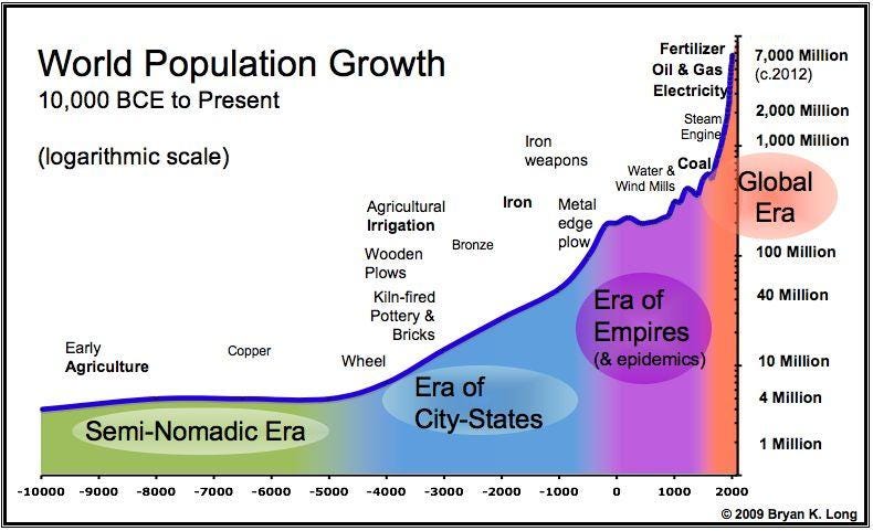
Human population didn’t start to explode until agriculture launched a feedback loop starting around 5000 BC. Surplus energy fed population growth, which freed up specialists who made discoveries that multiplied energy again, tightening the cycle until humanity’s doubling time fell from millennia to centuries to mere decades post industrial revolution.

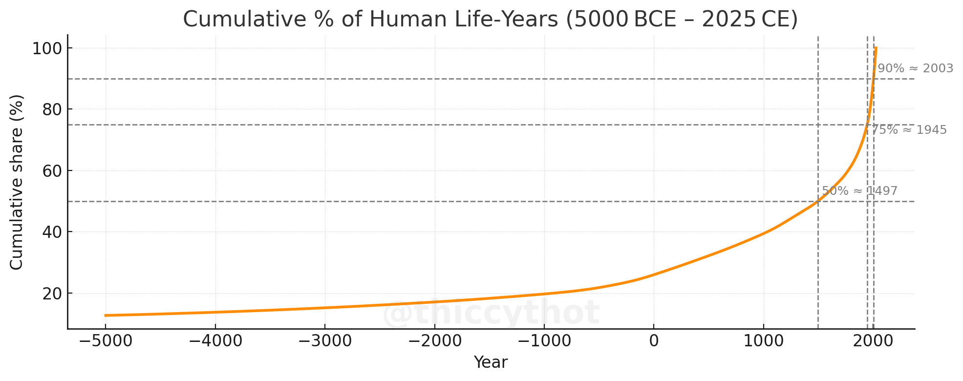
I charted the cumulative total of human life years by anchoring on known population figures from public datasets and linearly interpolated the gaps without introducing any assumptions about average lifespan (code below if you want to tweak the anchors).²

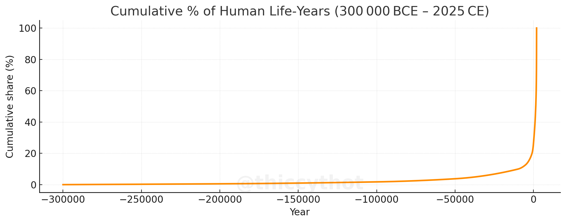
While the individual experiences time on a log scale, the collective has experienced time on an exponential scale, with almost eighty percent of human experience occurring in the last three millenia.

Zoom in and the view is even more extreme.

• 50% of all lived human experience occurs after 1500 CE

• 25% occurs after 1945 CE

• 10% occurs after 2003 CE

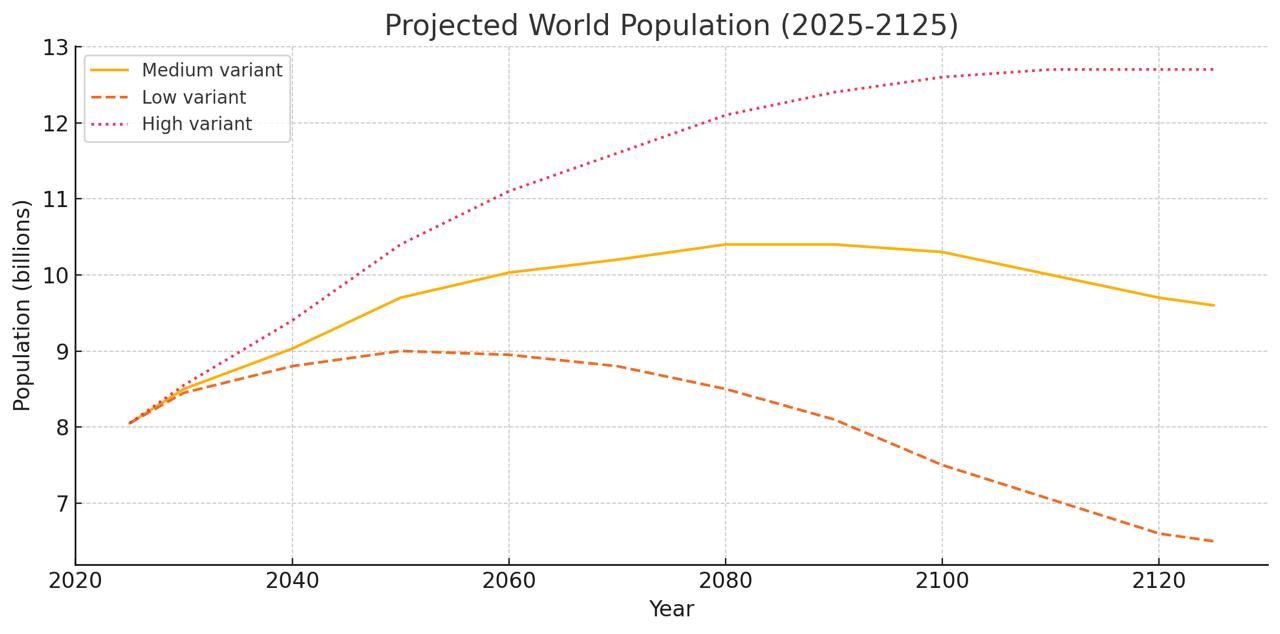
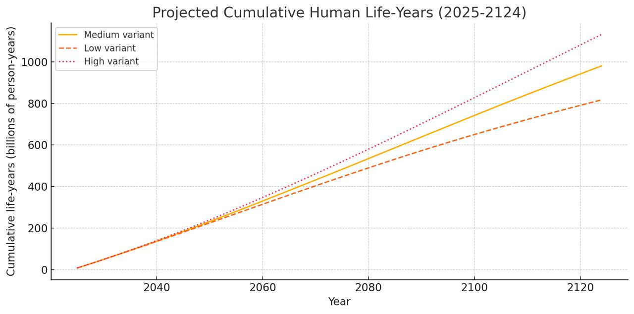
Even as global population is projected to top at ~10 billion 2080 as birthrates from developed nations naturally slow, there is still twenty five percent of all human experience that will be lived over the next 50 years. Every subsequent calendar year accounts for roughly 0.50% of all human experience.

The acceleration makes sense once you normalize by life-years, not by centuries. It’s one more “truth fractal” I keep bumping into: the idea that time is better counted in events than in objective time shows up in my day to day trading, stretches across an individual lifetime, and scales to the whole span of human history.

There’s plenty more of these fractals are out there. I’ll dig into them in future articles. Thanks for reading.

1. https://www.lesswrong.com/posts/SwBEJapZNzWFifLN6/the-funnel-of-human-experience

2

# ============================================================
#   CUMULATIVE HUMAN LIFE-YEARS   (300 000 BCE → 2025 CE)
#   — fully sourced anchor table + percentile plot —
# ============================================================
#
#  SOURCES (searchable):
#   • Schmidt, A. et al. 2021 – “Time dependence of population size in
#     Homo sapiens” – Nature 592: 195-200.                        [Schmidt2021]
#   • Scerri, E. et al. 2018 – “Did our species evolve in subdivided
#     populations across Africa?” – Trends in Ecology & Evolution 33(8). [Scerri2018]
#   • Durand, J.-D. 1974 – “Historical Estimates of World Population”,
#     Population Studies 28(2): 251-263.                           [Durand1974]
#   • Biraben, J.-N. 1980 – “Essai sur l’évolution du nombre des hommes”,
#     Population & Sociétés (HS): 1-48.                            [Biraben1980]
#   • Goldewijk, K. K. et al. 2017 – HYDE 3.3 historical database
#     of the global environment.                                  [HYDE2017]
#   • Maddison Project Database 2020 (Bolt & van Zanden).         [Maddison2020]
#   • United Nations, World Population Prospects 2022 revision.   [UNWPP2022]
#
#  Population numbers are in **millions** and deliberately rounded.
#  Deep-time genetic “effective population” values are scaled ×5
#  to approximate census head-counts.
# ============================================================

import numpy as np
import matplotlib.pyplot as plt

# -------------------------------
# Anchor population dictionary
# -------------------------------
anchor_pop_m = {
    # Deep pre-history (genetic / archaeological)
    -300_000: 0.07,  # Schmidt2021 Nature
    -200_000: 0.10,  # Scerri2018 TREE
    -100_000: 0.30,  # Durand1974 Population Studies
     -50_000: 1.00,  # Biraben1980 Pop & Soc – Upper Palaeolithic
     -10_000: 4.00,  # HYDE2017 10 000 BCE

    # 1 000-year grid 5000 → 1000 BCE  (HYDE2017)
      -5000: 14,  # 5000 BCE
      -4000: 20,  # 4000 BCE
      -3000: 27,  # 3000 BCE
      -2000: 35,  # 2000 BCE
      -1000: 50,  # 1000 BCE

    # 100-year grid −1000 BCE → 1500 CE (HYDE2017 unless stated)
      -1000: 50,  -900: 55,  -800: 60,  -700: 70,  -600: 80,
       -500: 100, -400: 110, -300: 120, -200: 140, -100: 170,
          1: 190,   100: 195,  200: 200,  300: 205,  400: 210,
        500: 210,   600: 220,  700: 230,  800: 240,  900: 250,
       1000: 265,  1100: 310, 1200: 360, 1300: 360, 1400: 350,
       1500: 460,  # Maddison2020

    # 50-year grid 1500 CE → 2025 CE (Maddison2020 → UNWPP2022)
       1550: 500, 1600: 550, 1650: 600, 1700: 600, 1750: 790,
       1800: 910, 1850: 1260, 1900: 1650, 1950: 2521,
       2000: 6080, 2025: 8000  # UN mid-year estimate
}

# -------------------------------
# Build annual population series
# -------------------------------
anchor_years = np.array(sorted(anchor_pop_m.keys()))
anchor_vals  = np.array([anchor_pop_m[y] for y in anchor_years])

years_full = np.arange(anchor_years[0], 2026)                 # −300 000 → 2025
pop_annual = np.interp(years_full, anchor_years, anchor_vals) # millions
pop_annual *= 1e6                                             # persons

# -------------------------------
# Cumulative life-years (% total)
# -------------------------------
cum_py  = np.cumsum(pop_annual)
cum_pct = cum_py / cum_py[-1] * 100

# -------------------------------
# Percentile years (zoom window)
# -------------------------------
percentiles = [50, 75, 90]
pct_years   = [int(years_full[np.searchsorted(cum_pct, p)]) for p in percentiles]

# -------------------------------
# Plot 1 – full 300 000 BCE → 2025 CE
# -------------------------------
plt.figure(figsize=(10,4))
plt.plot(years_full, cum_pct, color="darkorange", lw=2)
plt.title("Cumulative % of Human Life-Years (300 000 BCE – 2025 CE)")
plt.xlabel("Year")
plt.ylabel("Cumulative share of total life-years (%)")
plt.grid(True, ls=":", lw=0.4)
plt.tight_layout()
plt.show()

# -------------------------------
# Plot 2 – zoom 5000 BCE → 2025 CE with 50/75/90 %
# -------------------------------
mask = years_full >= -5000
plt.figure(figsize=(10,4))
plt.plot(years_full[mask], cum_pct[mask], color="darkorange", lw=2)

for p, yr in zip(percentiles, pct_years):
    plt.axhline(p, ls="--", c="gray", lw=1)
    plt.axvline(yr, ls="--", c="gray", lw=1)
    plt.text(yr + 25, p + 1.5, f"{p}% ≈ {yr}", color="gray", fontsize=8)

plt.title("Cumulative % of Human Life-Years (5000 BCE – 2025 CE)")
plt.xlabel("Year")
plt.ylabel("Cumulative share of total life-years (%)")
plt.grid(True, ls=":", lw=0.4)
plt.tight_layout()
plt.show()

print("Percentile crossover years:", dict(zip(percentiles, pct_years)))